6-DOF Robot Arm Simulator

Kinematics, trajectory planning, and a 3D viewer in Python, built from scratch

November 2025

This is a full simulation and control program for a six-axis robot arm, written in Python. I wrote the forward kinematics, inverse kinematics, trajectory planning, and 3D viewer myself, without any robotics libraries. The only dependencies are NumPy for the math and Matplotlib for the graphics.

The robot in the sim is modeled after the 6-DOF arm my brother Steve and I built. You can drive it two ways: click buttons to nudge the tool around a little at a time, or type in a command and watch it run a smooth move.

Goals

No robotics libraries: just NumPy and Matplotlib
Forward and inverse kinematics for a full 6-DOF arm
Two kinds of moves: fast joint moves, and straight-line moves where the tool follows a line in space
Interactive control: jog the tool from buttons, in either the world frame or the tool's own frame
Real-time 3D view showing where the tool is and which way it's pointing

Robot Model

The simulated arm has six rotating joints in the usual layout. J1 spins the whole arm around the vertical axis. J2 and J3 are the shoulder and elbow, which raise and lower the arm. The last three joints form a spherical wrist, so the tool can point any direction no matter where it is. The link lengths come straight from the real arm (191, 280, 92.5, 42, 310.5, and 56.5 mm), and fully stretched out it reaches about 700 mm.

I describe each joint with a screw axis instead of DH parameters. A screw axis for a rotating joint is two things: the direction it spins about (\(\omega\)), and any point on that axis (\(q\)). Those get packed into a single 6-vector:

S = \begin{bmatrix} \omega \\ v \end{bmatrix}, \qquad v = -\omega \times q

Here are the six axes at the home pose, with every joint at zero (all positions in mm):

Joint	Spins about (ω)	Point on the axis (q)
J1	z	(0, 0, 0)
J2	y	(42, 0, 191)
J3	y	(42, 0, 471)
J4	x	(42, 0, 563.5)
J5	y	(352.5, 0, 563.5)
J6	x	(409, 0, 563.5)

At home the upper arm points straight up, the forearm points straight out along x, and the tool sits at (409, 0, 563.5) mm. That home pose is the matrix \(M\).

Forward Kinematics

Forward kinematics answers a simple question: if I know all six joint angles, where's the tool?

With screw axes, the answer is the Product of Exponentials formula. You turn each joint's screw axis into a transform for its current angle, multiply all six together, and then multiply by the home pose:

T(\theta) = e^{[S_1]\theta_1}\, e^{[S_2]\theta_2} \cdots e^{[S_6]\theta_6}\, M

\(T\) comes out as a 4×4 matrix with the tool's orientation in the top-left 3×3 block (\(R\)) and its position in the last column (\(p\)). The screw-theory approach here follows Modern Robotics by Kevin Lynch and Frank Park.

Each exponential has a closed form. The rotation part is Rodrigues' formula, and the position part uses a matrix \(G\) that accounts for the point swinging around the axis:

\begin{aligned} R &= I + \sin\theta\,[\omega] + (1 - \cos\theta)\,[\omega]^2 \\ p &= \left( I\theta + (1 - \cos\theta)\,[\omega] + (\theta - \sin\theta)\,[\omega]^2 \right) v \end{aligned}

\([\omega]\) is the 3×3 skew-symmetric matrix of \(\omega\) (the matrix version of a cross product).

The same loop also builds the space Jacobian \(J_s\). Each column is that joint's screw axis, moved to wherever the joints before it have carried it:

\begin{aligned} J_{s1} &= S_1, \qquad J_{si} = \mathrm{Ad}_{T_{i-1}}\, S_i \\ T_{i-1} &= e^{[S_1]\theta_1} \cdots e^{[S_{i-1}]\theta_{i-1}} \end{aligned}

\(\mathrm{Ad}\) is the 6×6 adjoint matrix, built from the rotation and position of a transform. It re-expresses a screw axis in a new pose. The Jacobian tells you how the tool moves when the joints move: a small joint change \(\Delta\theta\) makes the tool move by the twist \(J_s\,\Delta\theta\). That's exactly what IK needs.

Inverse Kinematics

Inverse kinematics goes the other way: given where I want the tool and which way it should point, what joint angles get it there? That's a much harder problem. Sometimes there are several answers, sometimes there are none, and in general there's no neat formula.

So instead of solving it on paper, I wrote a numerical solver that uses Newton's method. It starts from the joint angles the arm has right now and keeps nudging them closer to the answer.

Pose error

A target is given as six numbers: a position (x, y, z) in mm and an orientation (rx, ry, rz) as an axis-angle vector in radians. The direction of that vector is the axis to rotate about, and its length is how far to rotate. Rodrigues' formula turns it into the goal transform \(T_d\).

Each iteration, the solver runs forward kinematics to get the tool's current pose \(T(\theta)\), and works out the transform that would carry it to the goal:

T_{\text{err}} = T_d\, T(\theta)^{-1}

Then it takes the matrix log of \(T_{\text{err}}\) to turn it into a 6-vector twist, the "how far and which way" of the error:

V_{\text{err}} = \log(T_{\text{err}}) = \begin{bmatrix} \omega_{\text{err}} \\ v_{\text{err}} \end{bmatrix}

\(\omega_{\text{err}}\) is the rotation the tool still needs (axis times angle, in radians), and \(v_{\text{err}}\) is the linear part, in mm. To take the log, you get the angle from the trace of the rotation, the axis from its skew-symmetric part, and the linear part by undoing \(G\):

\begin{aligned} \theta &= \arccos\!\left( \frac{\operatorname{tr}(R) - 1}{2} \right) \\ [\omega] &= \frac{R - R^{\mathsf T}}{2 \sin\theta} \\ v &= \left( \frac{I}{\theta} - \frac{[\omega]}{2} + \left( \frac{1}{\theta} - \frac{1}{2}\cot\frac{\theta}{2} \right) [\omega]^2 \right) p \end{aligned}

Newton step

The Jacobian says a joint change \(\Delta\theta\) moves the tool by \(J_s\,\Delta\theta\). We want that to equal the error, so we solve for \(\Delta\theta\) and take the step:

\Delta\theta = J_s^{+}\, V_{\text{err}}, \qquad \theta \leftarrow \theta + \Delta\theta

\(J_s^{+}\) is the pseudoinverse of the Jacobian. It matters here, because a plain inverse fails whenever the Jacobian is singular. That includes the home pose itself: with every joint at zero, J4 and J6 spin about the same line, so two columns of the Jacobian are identical. The pseudoinverse still gives the smallest step that does the best job of shrinking the error.

Since each step is based on a straight-line approximation of the arm, the first one won't land exactly on the target. So the solver repeats: run FK, measure the error, take a step. It stops once the rotation error is under 0.001 rad and the position error is under 0.001 mm. For poses the arm can reach, that usually takes under 30 iterations, and a single jog press takes about 2. If it still hasn't converged after 1,000 iterations, the solver gives up and raises an error, which usually means the pose is out of reach.

Once it converges, I wrap every joint angle back into −180° to 180°:

\theta = \operatorname{mod}(\theta + \pi,\ 2\pi) - \pi

Newton's method doesn't care how many full turns a joint has made, so without this the angles can drift off to values like 1,000°.

Starting from the arm's current joint angles turns out to be important. The arm can usually reach a pose several ways (elbow up or down, wrist flipped or not), and Newton's method tends to land on the solution closest to where it started. Seeding it with the current pose means the arm doesn't suddenly flip into a different configuration.

This is a different approach from the real arm. Steve's firmware uses a closed-form geometric solution that takes advantage of the spherical wrist. The numerical solver doesn't need any of that geometry, so it would work on any arm. The trade-off is that it's iterative, so it does more work per pose.

Trajectory Planning

Knowing the joint angles for a target isn't the whole story. The arm also needs a smooth way to get there. I wrote two kinds of moves, and both use a trapezoidal speed profile: speed up at a constant acceleration, cruise, then slow down at the same rate.

Joint moves (MoveJ)

A joint move is the quick, simple way to get from A to B. I solve IK once for the target, and then every joint runs its own trapezoidal profile from its start angle to its end angle.

First, each joint picks the shorter way around. If a joint needs to go +350°, it's quicker to go −10°, so the planner compares the change \(\Delta\theta\) with \(\Delta\theta - 2\pi\) (or \(\Delta\theta + 2\pi\)) and keeps whichever is smaller.

You give the move a total time \(T\). Each joint spends the first 10% of it speeding up and the last 10% slowing down:

t_a = 0.1\, T

Plotted against time, the speed is a trapezoid, and the area under it has to equal the distance the joint travels. That area works out to \(v\,(T - t_a)\), so each joint's top speed and acceleration are:

v = \frac{|\Delta\theta|}{T - t_a}, \qquad a = \frac{v}{t_a}

The joint angle over time is then three pieces:

\begin{aligned} \text{speeding up:} \quad & \theta(t) = \theta_{\text{start}} + \tfrac{1}{2} a t^2 \\ \text{cruising:} \quad & \theta(t) = \theta_{\text{start}} + \tfrac{1}{2} a t_a^2 + v\,(t - t_a) \\ \text{slowing down:} \quad & \theta(t) = \theta_{\text{end}} - \tfrac{1}{2} a\,(T - t)^2 \end{aligned}

Every joint uses the same \(T\) and \(t_a\), so they all start and stop at the same time. A joint with farther to go just gets a higher \(v\) and \(a\). The catch is that the tool doesn't follow a straight line. It takes whatever curved path falls out of the joints moving together.

Joint moves: every joint starts and stops together, and the tool follows a curved path

Linear moves (MoveL)

A linear move makes the tool travel in a straight line through space. That's what you want for things like welding or painting, or anywhere a surprise detour could hit something.

This time the profile is set by speed and acceleration limits instead of a time. The trapezoid applies to the distance \(d\) along the line. Speeding up from rest to \(v\) takes a distance \(d_a = v^2/(2a)\). If the move is long enough to fit both ramps, there's a cruise in the middle:

d \ge 2d_a: \quad t_a = \frac{v}{a}, \quad t_c = \frac{d - 2d_a}{v}

If it isn't, the arm never reaches \(v\). It speeds up for the first half and slows down for the second, a triangle instead of a trapezoid:

d < 2d_a: \quad t_a = \sqrt{d/a}, \quad t_c = 0, \quad v_{\text{peak}} = a\, t_a

Either way the move takes \(T = 2t_a + t_c\). At any moment, the distance covered so far divided by \(d\) gives a progress value \(s\) that goes from 0 to 1. Both position and orientation are driven by that same \(s\), so they start and finish together.

Position just slides along the line:

p(s) = p_{\text{start}} + s\,(p_{\text{end}} - p_{\text{start}})

For orientation, I find the single rotation that takes the start orientation to the end orientation, and pull its axis \(\hat\omega\) and total angle \(\theta_{\text{total}}\) out with the same trace formula as before:

R_{\text{rel}} = R_{\text{end}}\, R_{\text{start}}^{\mathsf T}

Then I sweep the angle from 0 to \(\theta_{\text{total}}\) while keeping the axis fixed:

R(s) = \mathrm{Rot}(\hat\omega,\ s\,\theta_{\text{total}})\, R_{\text{start}}

The tool turns smoothly at a steady rate about one fixed axis, instead of wobbling the way it can if you blend three separate angles.

Before the move starts, the planner splits the line into 100 steps and solves IK at each one. Each solve starts from the answer to the one before it, so neighboring solutions stay close together and the solver can't jump to a different arm configuration partway through. While the move runs, the sim works out \(s\) from the clock, finds which two waypoints it falls between, and blends their joint angles linearly. Between waypoints that's a joint-space blend, so the tool isn't perfectly on the line, but with 100 waypoints the difference is tiny.

The real arm doesn't do this orientation sweep yet: its firmware holds the tool's starting orientation for the whole move. That's one of the features I'd like to bring over.

	Simulator	Real arm firmware
Inverse kinematics	numerical (Newton's method)	closed-form, geometric
Speed profile	trapezoidal	S-curve
Orientation during a straight-line move	rotates smoothly from start to end	held at the start orientation

Visualization

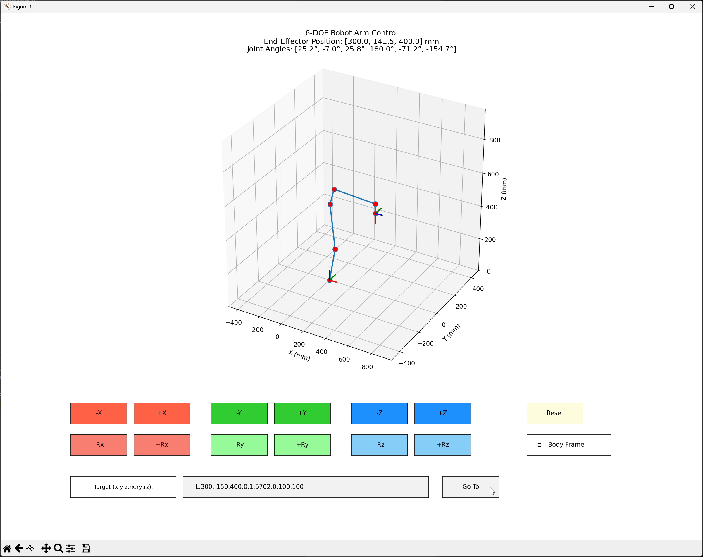
The robot shows up as a 3D stick figure, with a red sphere at each joint. The tool has a little RGB coordinate frame on it (red for X, green for Y, blue for Z), so you can see which way it's pointing. A matching frame at the origin shows the world axes for reference, the same way the real arm has an RGB axis triad on its end effector.

The view updates in real time. Moves are timed off the computer's clock, so a 2-second move really takes 2 seconds. The title bar shows the tool's current position and all six joint angles in degrees.

The simulator window with the 3D view, jog buttons and command box — The simulator, with the jog buttons and command box below the 3D view

Controls

There are two rows of jog buttons. The first row moves the tool: each press of +X moves it 10 mm along X, and the same goes for Y and Z. The second row rotates it, 5° per press about each axis. Every press is one IK solve, starting from the current joint angles.

A toggle switches between world frame and body frame. In world frame, +X always means the global X direction. In body frame, +X moves along the tool's own X axis, wherever that happens to be pointing. Body frame is the natural one for things like pushing the tool forward along its own axis.

The difference between the two comes down to which side you multiply the small rotation on. A 5° step \(\mathrm{Rot}\) gets applied to the tool's current orientation \(R\) like this:

\begin{aligned} \text{world frame:} \quad & R_{\text{new}} = \mathrm{Rot}\cdot R \\ \text{body frame:} \quad & R_{\text{new}} = R\cdot \mathrm{Rot} \end{aligned}

Multiplying on the left rotates about the world axes, and multiplying on the right rotates about the tool's own axes. Either way, the tool's position stays where it is, so it turns in place. (Multiplying the full pose \(T\) on the left would also swing the tool around the world origin.) For translation, world frame adds 10 mm along a global axis. Body frame adds 10 mm along one of the columns of the tool's rotation matrix, which are the tool's own axes.

Jogging in the world frame

Jogging in the body frame, where each move follows the tool's own axes

For full moves, there's a text box where you type commands:

J, x, y, z, rx, ry, rz, duration
L, x, y, z, rx, ry, rz, velocity, acceleration

J is a joint move and L is a linear move. Position is in mm, and orientation is given as an axis-angle vector in radians. A joint move takes a duration in seconds, and a linear move takes a velocity in mm/s and an acceleration in mm/s².

What's Next

Next, I want to turn this into a full robot simulator for our current robot arm.

Conclusion

This project covers the core of how a robot arm moves: forward kinematics to get the pose from the joint angles, inverse kinematics to get the joint angles from the pose, and trajectory planning to move smoothly between them. Being able to jog the arm around and actually watch it move made all of these ideas a lot less abstract. You can see right away what the arm can reach, and how a joint move and a linear move differ.

Thanks for reading!